Zero to Analytics from raw data to real insights in under 30 minutes

Setting up your first pipeline doesn’t have to mean days of setup or hours of configuration. With IOMETE, you can go from a raw file to actionable insights in minutes. To prove it, we’ll walk through an example with NYC taxi rides — a dataset big enough to be real, but simple enough to reason with.

Prerequisites

Before you start, make sure you have:

• A working setup of IOMETE
• Access to a running compute cluster and permissions to configure it
• Permissions to execute SQL queries, and to create databases and tables

If you don’t already have a running setup, you can ask your infrastructure team to follow the IOMETE on-prem installation guide.

Step 0: Get and upload the dataset

We’ll use two files published by the NYC Taxi & Limousine Commission:

• yellow_tripdata_2025-01.parquet
• taxi_zone_lookup.csv

Upload them into your default IOMETE storage (the system bucket created during install).

info

Using the default bucket means you don’t need to configure credentials — the default user already has access.

Optional: Use a different storage

If you want to point to a different S3-compatible storage instead, you can configure credentials in two ways:

At the session level (SQL Editor):

SET spark.hadoop.fs.s3a.bucket.<bucket-name>.endpoint=<endpoint-url>;
SET spark.hadoop.fs.s3a.bucket.<bucket-name>.access.key=<username>;
SET spark.hadoop.fs.s3a.bucket.<bucket-name>.secret.key=<password>;

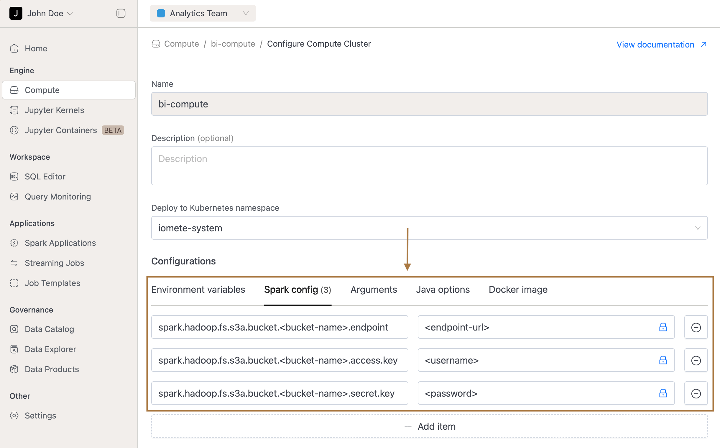
At the compute cluster level (UI): 1. Open Compute Cluster → Configure (terminate cluster in case it is already running). 2. Go to Spark Config. 3. Add your S3 endpoint, access key, and secret key. 4. Save and start the cluster.

Step 1: Create a database

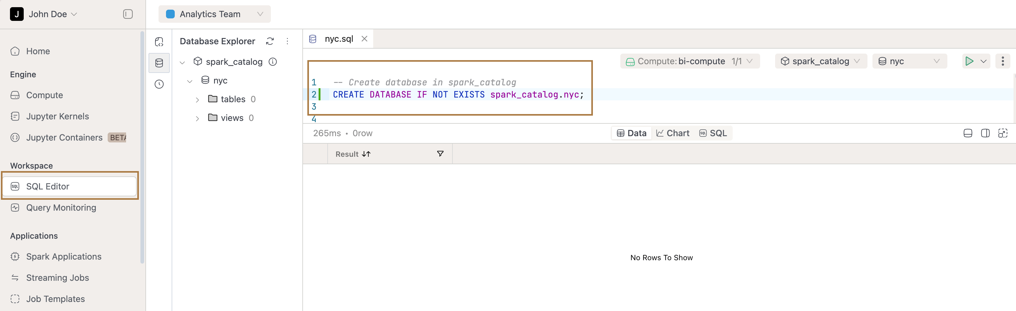
Open the SQL Editor and create a new worksheet. To keep things organized, we’ll create a dedicated database called nyc.

CREATE DATABASE IF NOT EXISTS spark_catalog.nyc;

This ensures that all tables you create in the following steps will live inside the nyc database, making your project easier to manage.

Step 2: Raw files → Iceberg tables

We’ll use the Parquet and CSV files to create Iceberg tables, as working directly with files isn’t user-friendly — you’d need to remember file paths, deal with inconsistent schemas, and even face latency issues if the files live in external storage.

-- Trips
CREATE OR REPLACE TABLE spark_catalog.nyc.yellow_trips_2025_01
USING iceberg
PARTITIONED BY (days(pickup_datetime))
AS
SELECT
  vendorid              AS vendor_id,
  tpep_pickup_datetime  AS pickup_datetime,
  tpep_dropoff_datetime AS dropoff_datetime,
  passenger_count,
  trip_distance,
  pulocationid          AS pu_location_id,
  dolocationid          AS do_location_id,
  payment_type,
  fare_amount,
  tip_amount,
  tolls_amount,
  congestion_surcharge,
  airport_fee,
  total_amount
FROM parquet.`s3a://iomete-system-bucket/nyc/yellow_tripdata_2025-01.parquet`;

-- Zone lookup
CREATE OR REPLACE TABLE spark_catalog.nyc.taxi_zone_lookup
USING iceberg
AS
SELECT
  CAST(_c0 AS INT)   AS location_id,
  _c1                AS borough,
  _c2                AS zone
FROM csv.`s3a://iomete-system-bucket/nyc/taxi_zone_lookup.csv`
WHERE _c0 != 'LocationID'; -- skip header row

Step 3: Clean and enrich → Fact table

The base trip table is useful, but still raw. It includes zero-minute trips, outliers, and missing values. If every analyst has to fix those in their own queries, results won’t be consistent.

That’s why we create a fact table: one place where data is cleaned and useful metrics are added. Everyone then works off the same definitions.

CREATE OR REPLACE TABLE spark_catalog.nyc.fct_trips_2025_01
USING iceberg
PARTITIONED BY (days(pickup_datetime))
AS
SELECT
  *,
  (unix_timestamp(dropoff_datetime) - unix_timestamp(pickup_datetime)) / 60.0 AS trip_minutes,
  CASE WHEN fare_amount > 0 THEN tip_amount / fare_amount END AS tip_rate,
  DATE(pickup_datetime)       AS pickup_date,
  HOUR(pickup_datetime)       AS pickup_hour,
  DATE_FORMAT(pickup_datetime, 'E') AS pickup_dow
FROM spark_catalog.nyc.yellow_trips_2025_01
WHERE trip_distance BETWEEN 0.1 AND 200
  AND total_amount BETWEEN 0 AND 1000
  AND dropoff_datetime >= pickup_datetime;

Now we’ve got a table with trustworthy metrics — trip_minutes, tip_rate, and clean date fields.

Step 4: Make it human-readable (add zone names)

Location IDs aren’t helpful in analysis. Let’s enrich the trips with readable borough and zone names from the lookup table.

CREATE OR REPLACE VIEW spark_catalog.nyc.v_trips_enriched AS
SELECT
  f.*,
  pu.borough AS pu_borough, pu.zone AS pu_zone,
  do.borough AS do_borough, do.zone AS do_zone
FROM spark_catalog.nyc.fct_trips_2025_01 f
LEFT JOIN spark_catalog.nyc.taxi_zone_lookup pu
  ON f.pu_location_id = pu.location_id
LEFT JOIN spark_catalog.nyc.taxi_zone_lookup do
  ON f.do_location_id = do.location_id;

Step 5: Create marts (ready-to-query)

Analysts often ask the same kinds of questions: when is demand highest, which routes are most profitable, how do people pay? Instead of rewriting GROUP BYs every time, we pre-aggregate marts for these use cases.

Hourly demand and revenue

CREATE OR REPLACE TABLE spark_catalog.nyc.m_hourly_zone_metrics
USING iceberg
AS
SELECT
  pickup_date,
  pickup_hour,
  pu_borough,
  pu_zone,
  COUNT(*)          AS trips,
  SUM(total_amount) AS revenue,
  SUM(tip_amount)   AS tips,
  AVG(tip_rate)     AS avg_tip_rate
FROM spark_catalog.nyc.v_trips_enriched
GROUP BY pickup_date, pickup_hour, pu_borough, pu_zone;

Top revenue routes

CREATE OR REPLACE TABLE spark_catalog.nyc.m_top_routes
USING iceberg
AS
SELECT
  pu_borough, pu_zone,
  do_borough, do_zone,
  COUNT(*)          AS trips,
  SUM(total_amount) AS revenue,
  AVG(tip_rate)     AS avg_tip_rate
FROM spark_catalog.nyc.v_trips_enriched
GROUP BY pu_borough, pu_zone, do_borough, do_zone
HAVING COUNT(*) >= 50
ORDER BY revenue DESC;

Payment mix

CREATE OR REPLACE TABLE spark_catalog.nyc.m_payment_mix
USING iceberg
AS
SELECT
  pickup_date,
  pickup_hour,
  CASE payment_type
    WHEN 1 THEN 'credit_card'
    WHEN 2 THEN 'cash'
    ELSE 'other'
  END AS payment_method,
  COUNT(*)          AS trips,
  SUM(total_amount) AS revenue
FROM spark_catalog.nyc.fct_trips_2025_01
GROUP BY pickup_date, pickup_hour, payment_method;

Step 6: Run queries for insights

Now the fun part — queries that deliver insights you’d actually share:

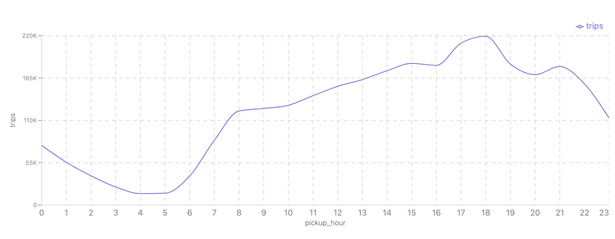
When does demand peak in Manhattan?

SELECT pickup_hour, SUM(trips) AS trips
FROM spark_catalog.nyc.m_hourly_zone_metrics
WHERE pu_borough = 'Manhattan'
GROUP BY pickup_hour
ORDER BY pickup_hour;

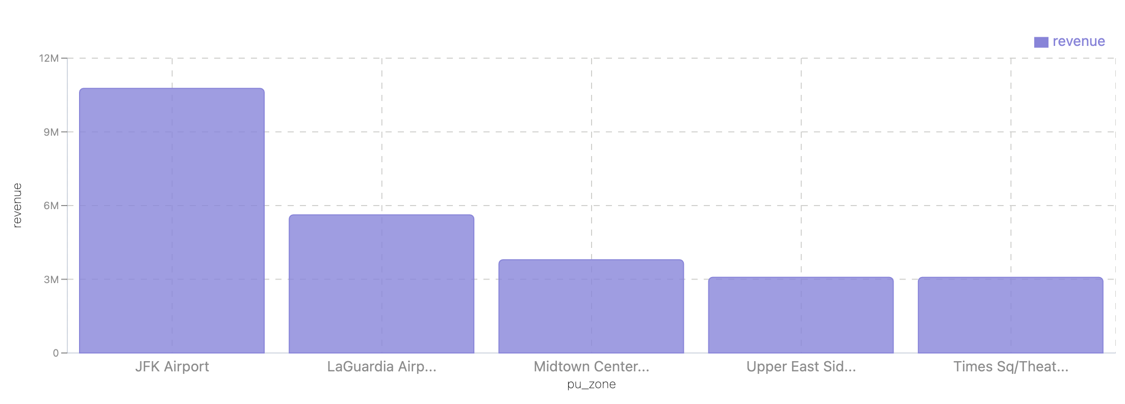
Which pick-up zones bring in the most revenue?

SELECT pu_zone, sum(revenue) as revenue
FROM spark_catalog.nyc.m_top_routes
GROUP BY pu_zone
ORDER BY revenue DESC
limit 5;

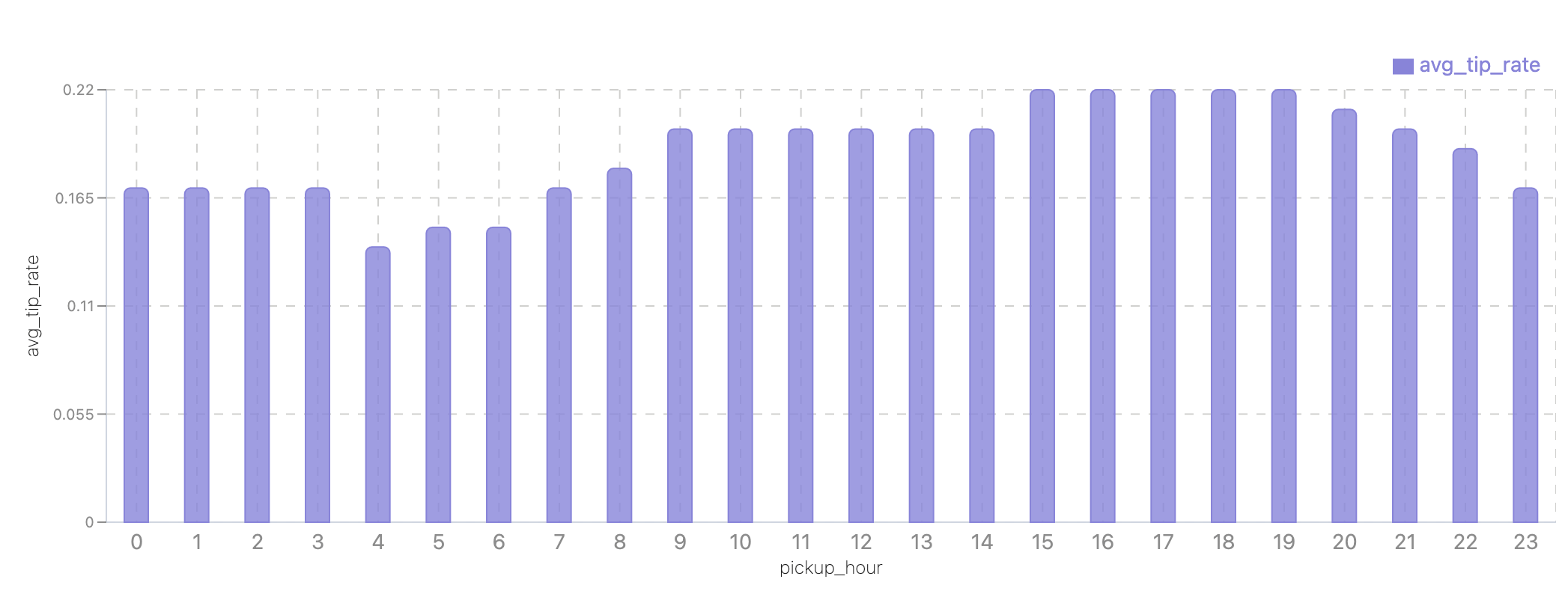
Do riders tip more at night?

SELECT pickup_hour, AVG(tip_rate) AS avg_tip_rate
FROM spark_catalog.nyc.fct_trips_2025_01
GROUP BY pickup_hour
ORDER BY pickup_hour;

End result

In less than 30 minutes, you:

• Created base tables from Parquet and CSV files, so you can work with them like proper tables instead of raw file paths.

• Built a fact table that cleaned up messy rows and added useful fields like trip_minutes, tip_rate, and calendar breakdowns.

• Published data marts for the most common questions: hourly demand, top routes by revenue, and payment mix.

With these three layers in place, you now have a small but complete pipeline: raw data → clean metrics → BI-ready tables.

The dataset we used was related to taxis, but the pattern applies everywhere. With IOMETE, you can follow the same steps for e-commerce orders, IoT logs, or financial transactions — and always get from raw files to insights quickly.

Next steps

• Automate transformations with dbt: model the fact + marts, schedule them, and add tests.

• Data Governance: Add validation & governance as you scale using data access policies.

• Time travel for audits: Use Iceberg time travel to reproduce dashboards exactly as they were at any point.