Apache Arrow

Apache Arrow has been taking the data world by storm over the last few years. In essence, it is a language-agnostic format designed for efficient in-memory storage and transfer of data. As such, it shares similarities with popular formats like JSON, Parquet, and XML.

Unlike other data formats, Arrow is optimized for fast processing of large datasets in memory. Its main goal is to eliminate serialization/deserialization overhead when transferring data between different systems written in various programming languages. It has the potential to become as foundational to data processing as HTTP/JSON is to web communication today.

In this article, we will explain how the Arrow format works and highlight the benefits of adopting it in modern data workflows.

Columnar vs Row-based formats

Apache Arrow is a columnar-based format, meaning data is stored by columns rather than rows. In a row-based format, like a spreadsheet, data is grouped by rows, which is great for tasks where you work with one record at a time. On the other hand, columnar formats like Arrow are ideal for analytical tasks, where you need to work with many rows but only a few columns. This structure makes it faster to process large amounts of data for analysis.

Row vs Column Storage: A LEGO Example

To help visualize this, imagine you have 100 LEGO castle kits and want to store the pieces in boxes. Storing them by rows is like keeping all the pieces needed to build one castle together in a box, just as you buy them in a shop. If you store them by column, it's like keeping all the pieces of the same color or size in separate boxes, with labels indicating which castle each piece belongs to.

Now, imagine you can only open one box at a time. If you want to build a single castle, it’s easier to grab the box with all the pieces for that castle. However if you want to count how many castles have no red pieces, it’s much quicker to open only the box with all red pieces (since all the red pieces were grouped together) versus looking through every box with pieces for each individual castle.

Row vs Column Storage: A Real-World Data Example

Let’s use a different sample set to visualize how data is laid out in memory between row-based and columnar formats. For this example, let’s consider a dataset with countries, their populations, and GDPs.

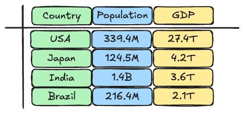
We’ll visualize memory as a straight line. In a row-oriented format, we store the data row by row. In a columnar format, we store the data for each column together.

The advantage of row-based data is that we can easily update an entire row by appending new data at the end, while invalidating the old row. However, if we want to perform an analysis — such as counting how many countries have a GDP over 4 trillion — we need to go through each row.

This is where columnar formats shine: with columnar storage, we can directly access the GDP data and quickly perform the analysis without needing to check every row.

Memory layout of the Arrow Columnar Format

Arrow offers a detailed specification on how it lays out buffers in memory or on disk. You can find the latest specification on the Arrow website: https://arrow.apache.org/docs/format/Columnar.html.

The core data structure in Arrow, recognized by all implementations, is called the Record Batch. A Record Batch consists of a Schema and ordered collections of Arrays.

• The Schema describes the structure of the dataset, including column names and data types. This metadata is serialized and stored using Google Flatbuffers. We won’t go into detail here on the schema, as this is just the metadata, and would require a deep dive into Flatbuffers.
• Each Array within a Record Batch holds values for only one datatype. Inside each array, there can be one or more Buffers. The number and type of buffers depend on the datatype and whether the data contains null values.

These buffers are contiguous regions of memory with a specific length in bytes. To visualize this, think of reserving 10 parking spaces in a parking garage. The term “contiguous” means that you reserve 10 spaces next to each other on the same floor, instead of scattered across different levels. This layout helps the CPU load the data more efficiently—similar to how it’s easier for a human to count if all reserved parking spaces are filled in one row, rather than spread across the garage.

Within each array, the buffers serve different purposes:

• Length buffer: This represents the number of values in the array.
• Null count buffer: This indicates the number of null values within the array.
• Validity bitmap: This is a series of 0s and 1s, which flags whether an entry in the array is semantically null (similar to knowing whether a data point has a known or unknown value).
• Value buffer: This contains the actual data values.
• Offset buffer: This helps locate the start and end positions of values in the value buffer.

Arrow Physical Layout: A Simple Example

Let’s go back to our example of countries and their population vs GDP numbers and make a simplified overview of the physical memory layout.

Each country has a name that will always be provided. This is a “variable length” format, as the length of the name is different for each country. So here we don’t need a validity bitmap, but we do get an offset buffer to help us find where each country’s name starts and ends in the value buffer.

The population data is something we can just grab from wikipedia. We would store this as fixed width 8 byte (i.e. 64 bits) numbers, which means we only need a value buffer here. As we have population data for each country, we don’t need a validity bitmap either.

Finally, we can also find GDP data on wikipedia. Similar to population data, we can use fixed width 8 byte numbers. However, we don’t have data for some countries, which means here we will add a validity bitmap.

Fixed-Size Primitive Data Type Example

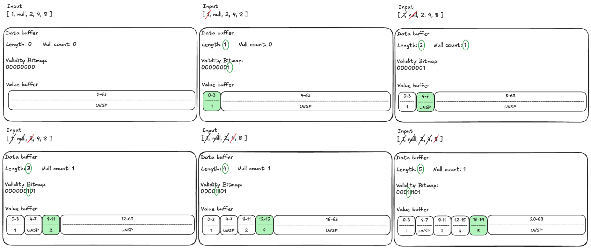
Let’s go over an example together. In the below, we start with an empty data buffer for an 32 bit integer value. Remember that 1 byte is 8 bits, so this is equivalent to saying a 4 byte integer value. We want to store the values 1, null, 2, 4 and 8.

In the first step, we want to add the value “1” from the input to the data buffer. To store the value, we reserve the first 4 bytes in the value buffer and place the value 1 in there. We now have 1 value in the data buffer, so we update the length to 1. Since we added a non-null value in the first place, we updated the right-most bit in the validity bitmap to 1.

In the next step, we want to add a null value. We reserve the next 4 bytes in the value buffer, and the exact value stored in there is up to the specific implementation. We then update the length of the buffer to 2 since we now have added two values. Since we added a null, we also increment the null count. Finally, we need to make sure the second right-most bit in the validity bitmap remains a 0 to indicate we have a semantic null as the second entry.

The remaining steps are similar to the steps above. In each step, we put the value in the value buffer, increment the length, and update the validity bitmap appropriately.

Variable-Size Data Type Example

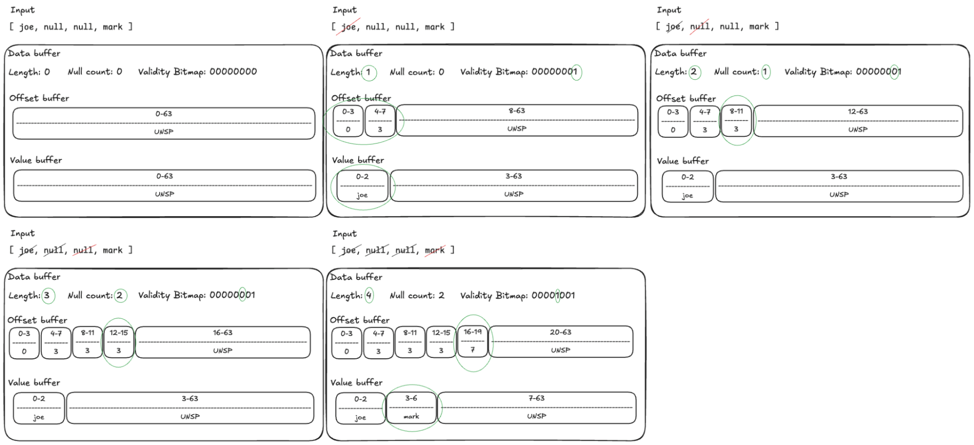
Let’s do one more example together, this time looking at variable width string data types. Assume we want to store the values joe, null, null and mark.

In the first step we want to add the word “joe” to our data buffer. This word will take 3 bytes to store in the value buffer, 1 byte per letter. We then update the offset to buffer to indicate the first word starts at index 0 and the next word starts at index 3. Then we update the length to 1, after which we set the right most bit in the validity bitmap to a 1.

In steps 2 and 3 we want to add a null value. In both cases, we do not touch the value buffer as there is no value to write. We set the end of each word to the same location as the latest start in the value buffer, which would be the same behavior if we would have received an empty string instead of a null value. Contrary to an empty string, we make sure the validity bitmap at the 2nd right most and, resp. the 3rd right most bit, in the validity bitmap is set to 0 to indicate that the value is null. We also increase the null count by 1 for each null. Finally, we bump the length by 1 for each null value we handle.

Lastly, we want to add the word mark. Will add 4 bytes to the value buffer. Then we add to the offset buffer that the next word, if added, would start at offset 7 in the value buffer. Then we set the 4th right most bit to a 1 in the validity bitmap, after which we increment the length by 1.

Other Arrow Data Types

Besides fixed and variable width data types, Arrow also supports lists, maps, structs, unions and more. The physical memory layout for each type is slightly different. The above examples should make it straightforward to understand how Arrow handles others. We recommend having a look over the specifications: https://arrow.apache.org/docs/format/Columnar.html#physical-memory-layout.

Key Advantages of Arrow

Arrow promises the following advantages:

• Data adjacency for sequential access (scans)
• O(1) (constant-time) random access
• SIMD and vectorization-friendly
• Relocatable without “pointer swizzling”, allowing for true zero-copy access in shared memory

These are all very technical sounding. Below we will dive into each of these to understand what they mean and how Apache Arrow delivers them.

Data Adjacency for Performance

To understand data adjacency (also known as data locality), we need some context on how CPU caches work. The specifics of these caches vary depending on the CPU architecture, but let's use a typical modern quad-core CPU as an example.

Think of the CPU as a kitchen, with each core being like an independent cooking island. Each cooking island needs easy access to the ingredients it will be using to prepare a dish.

• L1 cache is like the ingredients you have standing right next to your stove on the kitchen counter, ready to go. This cache is integrated with the CPU core, it’s the fastest to access and is typically 64KB in size.
• L2 cache is like the ingredients stored in a well-organized kitchen cabinet. You may need to open a cupboard, perhaps look around a bit, but you don’t have to walk away from the stove. On modern CPUs the L2 cache is also integrated with the CPU core but is slightly further away from the core itself. Typically it ranges from 256KB in older models to 16MB in high-end CPUs.
• L3 cache is like a shared kitchen pantry that all cooking islands use. You have to walk away from your cooking station to grab an ingredient, but it’s still within the kitchen. L3 cache is integrated with the CPU, but not the cores. It is shared between CPU cores, with sizes ranging from 2MB to 64MB.
• RAM is the main memory installed on your computer, much farther from the CPU than any of the caches. It is like the chef needing to do a round trip to the local supermarket to grab an ingredient.

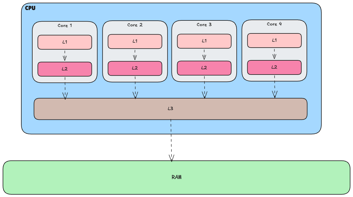
If the CPU is unable to find the data in a particular cache, it’s called a cache miss. The CPU will then fall back to other caches to look for the data. It ultimately tries to load the most frequently used data into the L1 cache. The CPU moves data up the hierarchy using cache lines, which are blocks of data typically 64 bytes in size on modern CPUs. The CPU grabs an entire 64-byte block, starting at what are known as cache line boundaries.

In our kitchen analogy, a cache miss is like not finding an ingredient on the stove and having to check the cabinets, pantry, or supermarket. Imagine Arrow as organizing ingredients by type—keeping all the flour in one box, all the sugar in another, and all the spices in a third. Cache line boundaries would be similar to grouping ingredients into manageable boxes that the chef can carry easily. When the chef needs flour, they can grab the entire box at once, maximizing efficiency by reducing the time spent searching through scattered items.

This is exactly how Apache Arrow optimizes memory layout for performance. By storing data in contiguous memory buffers, Arrow ensures that all the data for a particular value buffer is kept together in memory, reducing the need for the CPU to access scattered locations. This approach boosts data access speed and predictability, ensuring that related data is stored close together, thereby improving memory locality and overall performance. As a result, less CPU is needed overall.

O(1) Random Access

In computer science, Big O notation is used to describe the performance of algorithms relative to how the input data grows. For instance, a linear-time algorithm is O(n), which means the processing power needed increases linearly as the size of the data increases. This is similar to  if you need 5 people to do a job, so you can do 2 jobs at once with 10 people. If you get 3 more jobs to do at the same time, you will need to hire 15 more workers.

Arrow promises O(1) data access speeds. This means that no matter how much data there is, the speed at which you can access it remains consistent. To clarify, this doesn’t mean the access time itself is always the same, but rather that the size of the dataset doesn’t affect how quickly you can fetch data from it.

Let’s break this down with a simple example. Imagine we have a list of 5 numbers: [36, 12, 281, 6, 70]. Sorting these numbers by hand is easy. If we increase the size to 100 different numbers, you’d notice it takes more time. With 1000 numbers, sorting becomes even more time-consuming. The best sorting algorithms have a time complexity of O(n log n), meaning that as the dataset grows, the time taken to process it increases more than linear.

Now, instead of sorting numbers, imagine you’re asked to provide the number at position 3 in a list of 10 numbers. Even if the list has 100, 1000, or even a million numbers, it doesn’t affect how quickly you can retrieve the number at position 3. This is O(1)—constant time access, regardless of the size of the data.

How does Arrow achieve this? Let’s start with fixed-width data. As we saw in the serialization example above, we know that the value at the 3rd row will be located at bytes 8-11 in our value buffer. Retrieving this value is a simple operation. Similarly, for variable-width data, we first consult the offset buffer to determine where a string starts and ends. Once we know the location, accessing the actual data in the value buffer is straightforward.

So, no matter how large the dataset grows, accessing data from a specific column in a particular record is always done in constant time. Arrow prioritizes speed: by forgoing certain storage optimizations, like compression or complex data structures for deduplication, in favor of ensuring fast and consistent access times

SIMD Support and Vectorization in Arrow

SIMD is an acronym for Single Instruction, Multiple Data. It allows a CPU processor to process multiple data elements with a single CPU instruction, exploiting data-level parallelism. We will give a short overview of its power, for a more in depth read we suggest this article.

Imagine you have a block of cheese and a loaf of bread, and you want to make several cheese sandwiches. Without SIMD, you'd slice two pieces of bread, cut some cheese, assemble the sandwich, and repeat the process. With SIMD, it's like having a bread slicer that automatically slices the entire loaf into pieces in one go. Combining both bread and cheese in a single slicer would result in a mess, this is also why Arrow uses a columnar format: it groups bread with bread and cheese with cheese.Then having dedicated slicers for bread and cheese speeds up the entire sandwich-making process.

To understand the power of SIMD, we will use an example where we want to multiply the elements of two arrays. We choose C here because other languages tend to add overhead via various library calls. The most straightforward way to implement this would be to use a simple for loop to iterate through the arrays, multiply their corresponding elements, and store the results in a third array:

# define VECTOR_LENGTH 3

void _loop_multiply_vectors(int* v1, int* v2, int* v3) {
    for (int i = 0; i < VECTOR_LENGTH; i++) {
        v3[i] = v1[i] * v2[i];
    }
}

---

This gets compiled into the following CPU instructions

_loop_multiply_vectors:                 #@_loop_multiply_vectors
    mov     eax, dword ptr [rsi]
    imul    eax, dword ptr [rdi]
    mov     dword ptr [rdx], eax
    mov     eax, dword ptr [rsi + 4]
    imul    eax, dword ptr [rdi + 4]
    mov     dword ptr [rdx + 4], eax
    mov     eax, dword ptr [rsi + 8]
    imul    eax, dword ptr [rdi + 8]
    mov     dword ptr [rdx + 8], eax
    ret

---

For each iteration of the loop, the mov instruction moves an element from the first vector to the eax register. The imul instruction then multiplies the value in the register with the corresponding value from the second vector. Finally, another mov instruction stores the result back into the result vector. This sequence repeats for each element, and for an array of length 3, it generates 9 instructions (3 loads, 3 multiplications, and 3 stores, plus the loop control). If we increase the array length to 8, the total number of instructions increases to 24.

Let’s compare that using SIMD. To use SIMD, we need to use special data types. Here we will use the __m512i data type, where the 512 denotes we have a 512 bit wide registry and the “i” that the registry contains integer data types. We can see other available instructions for different CPU types on the Intel website.

The same code using SIMD look like:

__m512i _simd_multiply_vectors(__m512i v1, __m512i v2) {
    return _mm512_mullo_epi32(v1, v2);
}

---

This results in just a single CPU instruction to multiply the two vectors:

_simd_multiply_vectors:                 # @_simd_multiply_vectors
    vpmulld zmm0, zmm1, zmm0
    ret

---

This drastically reduces the number of operations needed to manipulate vectors. With a 512-bit wide register, we can process an entire 64-byte Arrow data buffer in one instruction. Arrow libraries, implemented in low-level languages like C++ and Rust, are designed to take advantage of SIMD operations internally, automatically optimizing data processing. Higher-level languages like Python and Java benefit from these optimizations without needing to explicitly handle SIMD instructions themselves..

To experiment with our C example yourself, you can use this link: https://godbolt.org/z/48xaKzxzG. These examples were compiled using the Clang compiler with the flags -O and -mavx512f. You'll notice that creating the SIMD data types introduces some overhead, but as the dataset size increases, this overhead becomes negligible compared to the number of operations required in a loop. In the case of Apache Arrow, the library ensures that data is made available in SIMD-friendly formats, so the optimizations can be leveraged automatically, even in higher-level languages.

Zero-Copy Access with Arrow: No Pointer Swizzling

This is a very technical sounding promise Arrow makes. Wikipedia defines pointer swizzling as “is the conversion of references based on name or position into direct pointer references (memory addresses)”.

To make sense of this, imagine two hospitals with their own incompatible software systems for storing patient information. If they want to share information about a patient, hospital A would print out a report containing the relevant details. This report would then be sent to hospital B, where a worker manually enters the information into their own system. What if you could just copy-paste the data from one system to the other like you can copy-paste between your iphone, ipad and macbook?

This type of process is common when different software systems or processes need to communicate. Despite being automated, these systems still rely on export, serialization, deserialization, and import steps to share data. Often these steps are custom written by Software Engineers working inside your company.

Arrow eliminates these steps. With a well-defined format, different processes and programming languages can directly operate on the same dataset. They don't even need to make local copies, and can share the data directly in shared memory.

Conclusion

In this article, we've only scratched the surface of what makes Apache Arrow a powerful choice for data analytics. We believe it has the potential to become the industry standard for powering large-scale data analytics.

The advantages of Arrow go beyond speed. By simplifying the exchange of data between different systems, it reduces the time, effort, and resources required for data interoperability. This opens up new possibilities for real-time data processing, data sharing, and cross-platform analysis. As data engineering and analytics continue to evolve, Apache Arrow is well-positioned to play a central role in shaping the future of data-intensive applications.