Migrating from Oracle to IOMETE/Spark

Migrating from Oracle to IOMETE/Spark: Performance Challenges and Solutions

TLDR

In this post, we'll share our real-world experience migrating Oracle queries to Spark/Iceberg, including the performance challenges we encountered and the strategies we used to overcome them.

Overview

One of our customers recently undertook a significant migration from their traditional Oracle data warehouse to a modern lakehouse architecture built on IOMETE. While modernizing their data platform was a key objective, they had an equally important requirement: ensuring their existing reports maintained or improved their performance levels.

Their legacy Oracle data warehouse ran on a powerful server with 64 CPUs and 500GB of RAM. In contrast, the new IOMETE Spark cluster was configured with 4 executors, each allocated 8 CPUs and 40GB of RAM—totaling 32 CPUs and 160GB of RAM across the cluster.

To establish a performance baseline, we executed approximately 50 reports of varying complexity on both systems. These reports represented their production workload and ranged from simple aggregations to complex multi-table joins. When run sequentially, the total execution time for all reports was:

	Total Execution Time
Oracle	24315 seconds (~6 hours 45 minutes)
IOMETE	1246 seconds (~20 minutes)

Despite Spark's impressive overall performance—completing all reports nearly 20x faster than Oracle—the customer wasn't entirely satisfied with the results. The reason? Oracle actually outperformed Spark on 17 individual reports.

This might seem contradictory at first glance: how could Spark be 20 times faster overall while losing on a third of the queries? The answer lies in the performance characteristics of each system. Spark excelled at complex, resource-intensive queries that previously took tens of minutes on Oracle, reducing them to mere seconds or minutes. However, Oracle maintained its advantage on lightweight, simple queries thanks to the B+Tree indexes on the tables.

In the next steps will reproduce similar case with synthetic data, and apply different techniques to improve the query performance of Spark.

Step 0: Building Testing Environment

Our performance analysis centered on two critical tables that appeared in nearly every query: inventory and catalog_items. Each table contained approximately 30 million rows and occupied roughly 400MB when stored as Parquet files on disk. To conduct meaningful performance comparisons, we replicated these table characteristics in our test environment, creating equivalent inventory and catalog_items iceberg tables that would serve as the foundation for our tests.

• catalog_items

  CREATE OR REPLACE TABLE catalog_items AS
  SELECT /*+ REPARTITION(5) */
    id                                                              AS item_id,
    CONCAT('Item_', item_id)                                        AS item_name,
    CONCAT('Category_', item_id % 10)                               AS category,
    ROUND(RAND() * 100, 2)                                          AS price,
    item_id % 2 = 0                                                 AS in_stock,
    CONCAT('Desc_', SUBSTRING(SHA1(CAST(item_id AS STRING)), 1, 8)) AS description,
    CONCAT('Brand_', item_id % 50)                                  AS brand,
    UPPER(SUBSTRING(SHA1(CAST(item_id * 17 AS STRING)), 1, 5))      AS sku_code
  FROM range(30000000);
• inventory

  CREATE OR REPLACE TABLE inventory AS
  SELECT /*+ REPARTITION(3) */
    id AS item_id,
    CAST(RAND() * 1000 AS INT) AS quantity_available,
    date_add(current_date(), CAST(rand() * -365 AS INT)) AS last_updated,
    CONCAT('Warehouse_', item_id % 5) AS location,
    CONCAT('Note_', SUBSTRING(SHA1(CAST(item_id + 99 AS STRING)), 1, 6)) AS notes
  FROM range(30000000);

To ensure our testing environment accurately mirrors production conditions, we repartitioned the data to generate Parquet files with sizes comparable to those in the live system.

The following query represents a typical customer report that we'll use as our optimization benchmark:

SELECT ci.*
FROM inventory AS inv
JOIN catalog_items AS ci USING (item_id)
WHERE inv.location = 'Warehouse_3'
  AND inv.last_updated BETWEEN CURRENT_DATE - 2 AND CURRENT_DATE
  AND inv.quantity_available < 10;

The report query demonstrates a classic analytical pattern: it retrieves detailed item information from the catalog_items table for a specific subset of items identified in the inventory table. In our test case, this selective query returns just ~100 rows from the 30-million-row datasets.

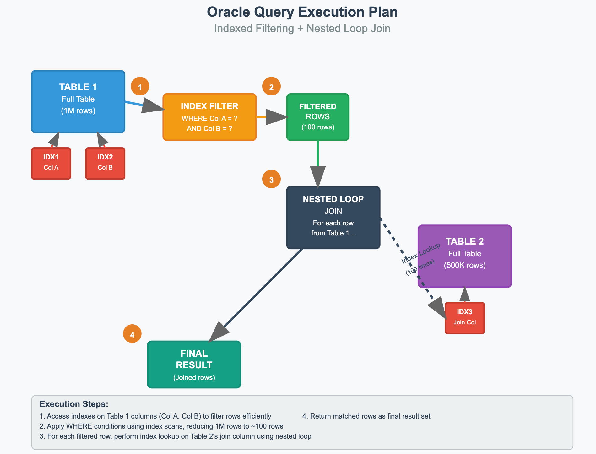
Traditional relational databases like Oracle excel at this type of selective query through their sophisticated indexing strategies. Oracle's execution plan follows an efficient two-step process: first, it uses indexes to rapidly filter the inventory table without scanning the entire dataset, then performs targeted index lookups on catalog_items based on the filtered results from step one. This index-driven approach eliminates the need for full table scans, enabling Oracle to return results in under 500 milliseconds with minimal disk I/O operations.

Step 1: Baseline - 7.3s

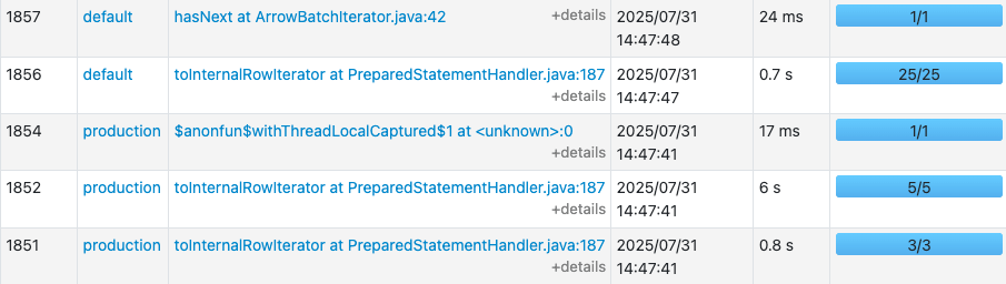
The query took 7.3s to finish in Spark. When we check Spark UI it is obvious that reading catalog_items table (Stage Id 1852) is the most dominant stage, which took 6s alone. It is as expected, but the unexpected part is its parallelism. It has been processed by only 5 tasks even though executors have 48 cores in total.

Thus, Spark executes the report much slower than Oracle (7.3s vs 0.5s), and we'll explore the root causes of this performance bottleneck and implement targeted optimizations to bridge this gap.

Step 2: Increased Parallelism - 3.5s

We will focus on the slowest stage - 1852 in this step, and try to make it faster. The catalog_items table has 5 parquet files each with size a bit less than 128mb row group size. So, each file is being processed by a single task, and as a result we get 5 tasks at that stage. We will recreate the table with more files but smaller size.

INSERT OVERWRITE catalog_items
SELECT /*+ REPARTITION(48) */
  *
FROM catalog_items;

-- Using the new catalog_items_smaller_files table
-- Duration: 3.5s
SELECT ci.*
FROM inventory AS inv
JOIN catalog_items AS ci USING (item_id)
WHERE inv.location = 'Warehouse_3'
  AND inv.last_updated BETWEEN CURRENT_DATE - 2 AND CURRENT_DATE
  AND inv.quantity_available < 10;

Catalog_items table get 48 files, each around 12MB size. The report finished in 3.5 seconds.

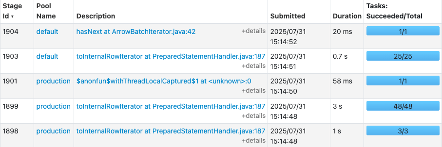
Now the slowest stage (1899) took 3s instead of 6s in the previous run due to number of tasks increased from 5 to 48.

Step 3: Wide table - 1.2s

Oracle achieves its performance through indexes—auxiliary data structures that enable rapid lookups but come with significant trade-offs. These indexes consume substantial disk space (often exceeding the table size itself) and degrade write performance due to maintenance overhead. In contrast, Spark operates purely on table data without additional structures. Moreover, the iceberg tables in IOMETE are 3x smaller than in Oracle.

Given these fundamental differences, we decided to create a denormalized wide table by pre-joining inventory and catalog_items for interactive reporting. This approach leverages columnar storage advantages: while wide tables are inefficient in row-oriented databases due to full-scan penalties, columnar formats like Parquet only read the specific columns needed for each query, making table width irrelevant to performance.

CREATE OR REPLACE TABLE inventory_catalog
AS
SELECT
  ci.*,
  inv.quantity_available,
  inv.last_updated,
  inv.location,
  inv.notes
FROM catalog_items AS ci
JOIN inventory AS inv USING(item_id);

-- Duration: 1.2s
SELECT
  *
FROM inventory_catalog AS inv
WHERE location = 'Warehouse_3'
  AND inv.last_updated BETWEEN CURRENT_DATE - 2 AND CURRENT_DATE
  AND inv.quantity_available < 10;

The denormalized table delivered immediate results: query execution time dropped to 1.2 seconds—a 6x improvement over the original 7.3-second performance. While this 1.2-second response time meets customer acceptance criteria, we'll implement additional optimizations in the next step to further close the gap with Oracle's sub-500ms baseline.

Step 4: Z-Order

We’ve already achieved sufficient performance, but will try to optimize further. Lets check the execution metrics of the execution plan of the Step 3:

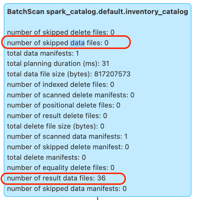
The wide table contains 36 Parquet files, and the query ended up reading all of them (skipped data files: 0).

According to the documentation, Parquet files store column statistics—such as min/max values—which can be used to skip unnecessary files during filtering. However, as shown in the execution details, the query engine did not skip any files.

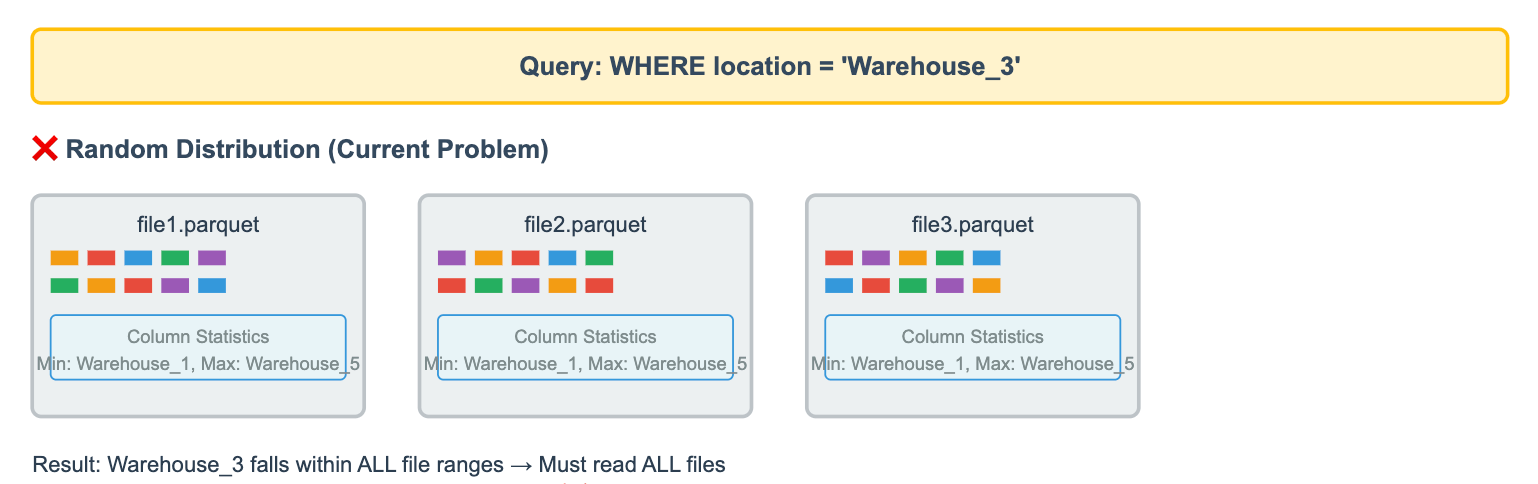
The reason is that the data was written to the table in a random distribution. For example, rows with location = Warehouse_3 can be scattered across any file. Even if a file contains no rows for Warehouse_3, it might still contain rows for Warehouse_2 and Warehouse_5. In such cases, the stored statistics might show:

min = Warehouse_2
max = Warehouse_5

Since Warehouse_3 falls within that range, the query engine cannot safely skip the file. As a result, it must open and read all 36 files.

The same limitation applies to other columns used in the WHERE clause.

If we organize the data to minimize each file’s min/max range for relevant columns, the query engine can more effectively skip unnecessary files.

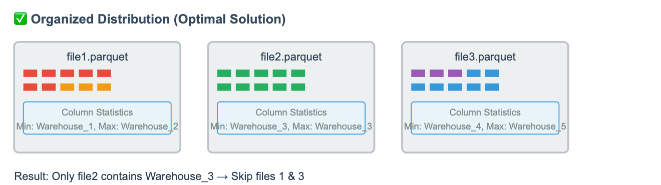
Then, lets re-organize the table by sorted order based on location and last_updated columns, and run the report again.

ALTER TABLE inventory_catalog WRITE ORDERED BY (location, last_updated);

INSERT OVERWRITE inventory_catalog
SELECT
  *
FROM inventory_catalog;

-- Duration: 0.5s
SELECT
  *
FROM inventory_catalog AS inv
WHERE location = 'Warehouse_3'
  AND inv.last_updated BETWEEN CURRENT_DATE - 2 AND CURRENT_DATE
  AND inv.quantity_available < 10;

The report query finished even faster - in 0.5 seconds! Lets review the query execution metrics.

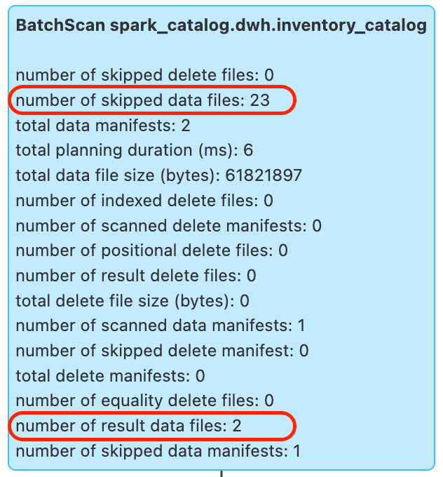
The query skipped 23 out of 25, and read only 2 parquet files!

Summary

Although Spark was originally designed for large-scale batch processing, we’ve explored practical techniques that enable sub-second interactive reporting. Key takeaways include:

• File sizing matters: Spark delivers the best throughput with large (256–512 GB) Parquet files. However, for smaller tables or latency-sensitive queries, generating smaller files can significantly reduce response times.
• Pre-join for speed: Build wide tables by pre-joining frequently accessed datasets. This reduces on-the-fly joins and accelerates interactive queries.
• Partition strategically: Apply partitioning where it aligns with query patterns to prune unnecessary data scans.
• Leverage sorting: Sort (or Z-order) data by columns commonly used in filters to maximize data skipping and improve query performance.